1.Introduction
This page explains how to use the PVGIS web interface to produce calculations of solar radiation and photovoltaic (PV) system energy production. We will try to show how to use PVGIS in practice. You can also have a look at the methods used to make the calculations or at a brief "getting starting" guide.
This manual describes PVGIS version 5.
1.1 What is PVGIS
PVGIS is a web application that allows the user to get data on solar radiation and photovoltaic (PV) system energy production, at any place in most parts of the world. It is completely free to use, with no restrictions on what the results can be used for, and with no registration necessary.
PVGIS can be used to make a number of different calculations. This manual will describe each of them. To use PVGIS you have to go through a few simple steps. Much of the information given in this manual can also be found in the Help texts of PVGIS.
1.2 Input and output in PVGIS
The PVGIS user interface is shown below.

Most of the tools in PVGIS require some input from the user - this is handled as normal web forms, where the user clicks on options or enters information, such as the size of a PV system.
Before entering the data for the calculation the user must select a geographical location for which to make the calculation. This is done by:
- By clicking on the map, perhaps also using the zoom option.
- By entering an address in the "address" field below the map
- By entering latitude and longitude in the fields below the map. Latitude and longitude can be input in the format DD:MM:SSA where DD is the degrees, MM the arc-minutes, SS the arc-seconds and A the hemisphere (N, S, E, W). Latitude and longitude can also be input as decimal values, so for instance 45°15'N should be input as 45.25. Latitudes south of the equator are input as negative values, north are positive. Longitudes west of the 0° meridian should be given as negative values, eastern values are positive.
PVGIS allows the user to get the results in a number of different ways:
- As number and graphs shown in the web browser. All graphs can also be saved to file.
- As information in text (CSV) format. The output formats are described separatelly in the "Tools" section.
- As a PDF document, available after the user has clicked to show the results in the browser.
- Using the non-interactive PVGIS web services (API services). These are described further in the "Tools" section.
2. Using horizon information
The calculation of solar radiation and/or PV performance in PVGIS can use information about the local horizon to estimate the effects of shadows from nearby hills or mountains. The user has a number of choices for this option, which are shown to the right of the map in the PVGIS tool.

The user has three choices for the horizon information:
- Do not use the horizon information for the calculations. This is the choice when the user unselects both the "calculated horizon" and the "upload horizon file" options.
- Use the PVGIS built-in horizon information. To choose this, select "Calculated horizon" in the PVGIS tool. This is the default option.
- Upload your own information about the horizon height. The horizon file to be uploaded to our web site should be a simple text file, such as you can create using a text editor (such as Notepad for Windows), or by exporting a spreadsheet as comma-separated values (.csv). The file name must have the extensions '.txt' or '.csv'. In the file there should be one number per line, with each number representing the horizon height in degrees in a certain compass direction around the point of interest. The horizon heights in the file should be given in a clockwise direction starting at North; that is, from North, going to East, South, West, and back to North. The values are assumed to represent equal angular distance around the horizon. For instance, if you have 36 values in the file, PVGIS assumes that the first point is due north, the next is 10 degrees east of north, and so on, until the last point, 10 degrees west of north. An example file can be found here. In this case, there are only 12 numbers in the file, corresponding to a horizon height for every 30 degrees around the horizon.
Most of the PVGIS tools (except the hourly radiation time series) will display a graph of the horizon together with the results of the calculation. The graph is shown as a polar plot with the horizon height in a circle. The next figure shows an example of the horizon plot. A fisheye camera picture of the same location is shown for comparison.

3. Choosing solar radiation database
The solar radiation databases (DBs) available in PVGIS are:
|
Database |
Type |
Start Year |
End Year |
Spatial res. |
Comments |
|
PVGIS-SARAH2 |
Satellite |
2005 |
2020 |
0.05° x 0.05° (~ 5 km) |
Default DB for Europe, Asia, Africa and South America (below 20 S) |
|
PVGIS-NSRDB |
Satellite |
2005 |
2015 |
0.038° x 0.0.38° (~ 4 km) |
Default DB for the Americas (above 20 S) |
|
PVGIS-ERA5 |
Reanalysis |
2005 |
2020 |
0.25° x 0.25° (~ 25 km) |
Default DB for rest of the world without coverage from satellite-based DBs |
|
PVGIS-SARAH |
Satellite |
2005 |
2016 |
0.05° x 0.05° (~ 5 km) |
This operational database is not updated any more. Please, use PVGIS-SARAH2 instead. |
All databases provide hourly solar radiation estimates.
Most of the solar radiation data used by PVGIS have been calculated from satellite images. There exist a number of different methods to do this, based on which satellites are used. The choices that are available in PVGIS at present are:
- PVGIS-SARAH2 This data set has been calculated by CM SAF to replace SARAH-1. This data cover Europe, Africa, most of Asia, and parts of South America.
- PVGIS-NSRDB This data set has been provided by the National Renewable Energy Laboratory (NREL) and is part of the National Solar Radiation Database.
- PVGIS-SARAH This data set was calculated by CM SAF and the PVGIS team. This data has a similar coverage than PVGIS-SARAH2.
Some areas are not covered by the satellite data, this is especially the case for high-latitude areas. We have therefore introduced an additional solar radiation database for Europe, which includes northern latitudes:
- PVGIS-ERA5 This is an reanalysis product from ECMWF. Coverage is worldwide at hourly time resolution and a spatial resolution of 0.28° lat/lon.
More information about the reanalysis-based solar radiation data is available.
For each calculation option in the web interface, PVGIS will present the user with a choice of the databases that cover the location chosen by the user.
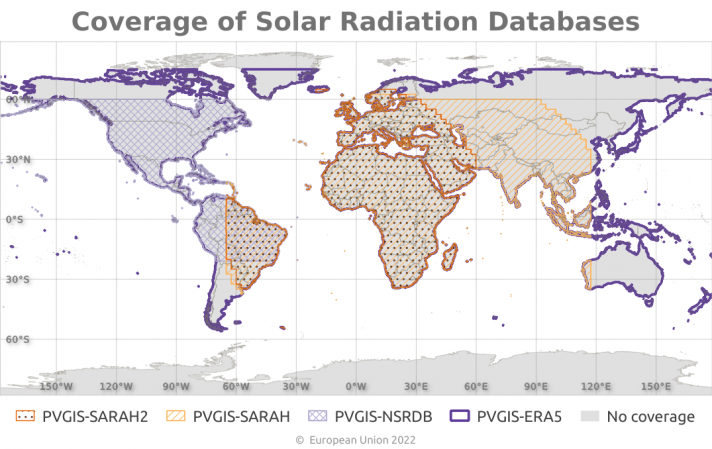
The figure below shows the areas covered by each of the solar radiation databases.
Based on the different validation studies performed the databases recommended for each location are the following:
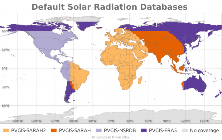
These databases are the ones used by default when the raddatabase parameter is not provided in the non-interactive tools. These are also the databases used in the TMY tool.
4. Calculating grid-connected PV system performance
Photovoltaic systems convert the energy of sunlight into electric energy. Although PV modules produce direct current (DC) electricity, often the modules are connected to an Inverter which converts the DC electricity into AC, which can then be used locally or sent to the electricity grid. This type of PV system is called grid-connected PV. The calculation of the energy production assumes that all the energy that is not used locally can be sent to the grid.
4.1 Inputs for the PV system calculations
PVGIS needs some information from the user to make a calculation of the PV energy production. These inputs are described in the following:

| PV Technology |
The performance of PV modules depends on the temperature and on the solar irradiance, but the exact dependence varies between different types of PV modules. At the moment we can estimate the losses due to temperature and irradiance effects for the following types of modules: crystalline silicon cells; thin film modules made from CIS or CIGS and thin film modules made from Cadmium Telluride (CdTe). For other technologies (especially various amorphous technologies), this correction cannot be calculated here. If you choose one of the first three options here the calculation of performance will take into account the temperature dependence of the performance of the chosen technology. If you choose the other option (other/unknown), the calculation will assume a loss of 8% of power due to temperature effects (a generic value which has found to be reasonable for temperate climates). PV power output also depends on the spectrum of the solar radiation. PVGIS can calculate how the variations of the spectrum of sunlight affects the overall energy production from a PV system. At the moment this calculation can be done for crystalline silicon and CdTe modules. Note that this calculation is not yet available when using the NSRDB solar radiation database. |
|
| Installed peak power |
This is the power that the manufacturer declares that the PV array can produce under standard test conditions (STC), which are a constant 1000W of solar irradiation per square meter in the plane of the array, at an array temperature of 25°C. The peak power should be entered in kilowatt-peak (kWp). If you do not know the declared peak power of your modules but instead know the area of the modules and the declared conversion efficiency (in percent), you can calculate the peak power as power = area * efficiency / 100. See more explanation in the FAQ. Bifacial modules: PVGIS doesn't make specific calculations for bifacial modules at present. Users who wish to explore the possible benefits of this technology can input the power value for Bifacial Nameplate Irradiance. This can also be can also be estimated from the front side peak power P_STC value and the bifaciality factor, φ (if reported in the module data sheet) as: P_BNPI = P_STC * (1 + φ * 0.135). NB this bifacial approach is not appropriate for BAPV or BIPV installations or for modules mounting on a N-S axis i.e. facing E-W. |
|
| System loss |
The estimated system losses are all the losses in the system, which cause the power actually delivered to the electricity grid to be lower than the power produced by the PV modules. There are several causes for this loss, such as losses in cables, power inverters, dirt (sometimes snow) on the modules and so on. Over the years the modules also tend to lose a bit of their power, so the average yearly output over the lifetime of the system will be a few percent lower than the output in the first years. We have given a default value of 14% for the overall losses. If you have a good idea that your value will be different (maybe due to a really high-efficiency inverter) you may reduce this value a little. |
|
| Mounting position |
For fixed (non-tracking) systems, the way the modules are mounted will have an influence on the temperature of the module, which in turn affects the efficiency. Experiments have shown that if the movement of air behind the modules is restricted, the modules can get considerably hotter (up to 15°C at 1000W/m2 of sunlight). In PVGIS there are two possibilities: free-standing, meaning that the modules are mounted on a rack with air flowing freely behind the modules; and building- integrated, which means that the modules are completely built into the structure of the wall or roof of a building, with no air movement behind the modules. Some types of mounting are in between these two extremes, for instance if the modules are mounted on a roof with curved roof tiles, allowing air to move behind the modules. In such cases, the performance will be somewhere between the results of the two calculations that are possible here. |
|
| Slope of PV modules |
This is the angle of the PV modules from the horizontal plane, for a fixed (non-tracking) mounting. For some applications the slope and azimuth angles will already be known, for instance if the PV modules are to be built into an existing roof. However, if you have the possibility to choose the slope and/or azimuth, PVGIS can also calculate for you the optimal values for slope and azimuth (assuming fixed angles for the entire year).
 |
|
| Azimuth (orientation) of PV modules |
The azimuth, or orientation, is the angle of the PV modules relative to the direction due South. - 90° is East, 0° is South and 90° is West. For some applications the slope and azimuth angles will already be known, for instance if the PV modules are to be built into an existing roof. However, if you have the possibility to choose the slope and/or azimuth, PVGIS can also calculate for you the optimal values for slope and azimuth (assuming fixed angles for the entire year).
 of PV modules") |
|
| Optimizing slope (and maybe azimuth) |
If you click to choose this option, PVGIS will calculate the slope of the PV modules that gives the highest energy output for the whole year. PVGIS can also calculate the optimum azimuth if desired. These options assume that the slope and azimuth angles stay fixed for the entire year. |
|
| PV electricity cost calculation |
For fixed-mounting PV systems connected to the grid PVGIS can calculate the cost of the electricity generated by the PV system. The calculation is based on a "Levelized Cost of Energy" method, similar to the way a fixed-rate mortgage is calculated. You need to input a few bits of information to make the calculation:
The calculation assumes that there will be a fixed cost per year for maintenance of the PV system (such as replacement of components that break down), equal to 2% of the original cost of the system. |
|
4.2 Calculation outputs for the PV grid-connected system calculation
The outputs of the calculation consist of annual average values of energy production and in-plane solar irradiation, as well as graphs of the monthly values.

In addition to the annual average PV output and the average irradiation, PVGIS also reports the year-to-year variability in the PV output, as the standard deviation of the yearly values over the period with solar radiation data in the chosen solar radiation database. You also get an overview of the different losses in the PV output caused by various effects.
When you make the calculation the visible graph is the PV output. If you let the mouse pointer hover above the graph you can see the monthly values as numbers. You can switch between the graphs clicking on the buttons:

Graphs have a download button in the top right corner. In addition, you can download a PDF document with all the information shown in the calculation output.
5. Calculating sun-tracking PV system performance
5.1 Inputs for the tracking PV calculations
The second "tab" of PVGIS 5 lets the user make calculations of the energy production from various types of sun-tracking PV systems. Sun-tracking PV systems have the PV modules mounted on supports that move the modules during the day so the modules face in the direction of the sun. The systems are presumed to be grid-connected, so the PV energy production is independent of local energy consumption.
6. Calculating off-grid PV system performance
6.1 Inputs for the off-grid PV calculations
PVGIS needs some information from the user to make a calculation of the PV energy production.
These inputs are described in the following:
|
Installed peak power |
This is the power that the manufacturer declares that the PV array can produce under standard test conditions, which are a constant 1000W of solar irradiation per square meter in the plane of the array, at an array temperature of 25°C. The peak power should be entered in watt-peak (Wp). Note the difference from the grid-connected and tracking PV calculations where this value is assumed to be in kWp. If you do not know the declared peak power of your modules but instead know the area of the modules and the declared conversion efficiency (in percent), you can calculate the peak power as power = area * efficiency / 100. See more explanation in the FAQ. |
| Battery capacity |
This is the size, or energy capacity, of the battery used in the off-grid system, measured in watt-hours (Wh). If instead you know the battery voltage (say, 12V) and the battery capacity in Ah, the energy capacity can be calculated as energy capacity=voltage*capacity. The capacity should be the nominal capacity from fully charged to fully discharged, even if the system is set up to disconnect the battery before becoming fully discharged (see next option). |
| Discharge cut-off limit |
Batteries, especially lead-acid batteries, degrade quickly if they are allowed to completely discharge too often. Therefore a cut-off is applied so that the battery charge cannot go below a certain percentage of full charge. This should be entered here. The default value is 40% (corresponding to lead-acid battery technology). For Li-ion batteries the user can set a lower cut-off e.g. 20%. |
| Consumption per day |
This is the energy consumption of all the electrical equipment connected to the system during a 24 hour period. PVGIS assumes that this daily consumption is distributed discretely over the hours of the day, corresponding to a typical home use with most of the consumption during the evening. The hourly fraction of consumption assumed by PVGIS is shown below and the data file is available here. 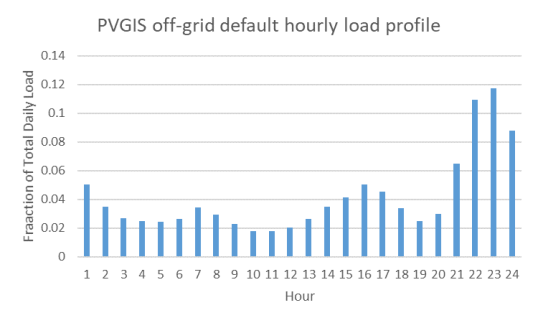 EC |
| Upload consumption data |
If you know that the consumption profile is different from the default one (see above) you have the option of uploading your own. The hourly consumption information in the uploaded CSV file should consist of 24 hourly values, each on its own line. The values in the file should be the fraction of the daily consumption that takes place in each hour, with the sum of the numbers equal to 1. The daily consumption profile should be defined for the standard local time, without consideration of daylight saving offsets if relevant to the location. The format is the same as the default consumption file. |
5.2 Calculation outputs for the off-grid PV calculations
PVGIS calculates the off-grid PV energy production taking into account the solar radiation for every hour over a period of several years. The calculation is done in the following steps:
- For every hour calculate the solar radiation on the PV module(s) and the corresponding PV power
- If the PV power is greater than the energy consumption for that hour, store the rest of the energy in the battery.
- If the PV power is less than the energy consumption, get the missing energy from the battery.
- If the battery becomes full, calculate the energy "wasted" i.e. the PV power could be neither consumed nor stored.
- If the battery becomes empty, calculate the missing energy and add the day to the count of days on which the system ran out of energy.
The outputs for the off-grid PV tool consist of annual statistical values and graphs of monthly system performance values. There are three different monthly graphs:
- Monthly average of the daily energy output as well as the daily average of the energy not captured because the battery became full
- Monthly statistics on how often be battery became full or empty during the day.
- Histogram of the battery charge statistics
These are accessed via the buttons:

Please note the following for interpreting the off-grid results:
i) PVGIS does all the calculations hour by hour over the complete time series of solar radiation data used. For example, if you use PVGIS-SARAH2 you will be working with 15 years of data. As explained above, the PV output is estimated.for every hour from the received in-plane irradiance. This energy goes directly to the load and if there is an excess, this extra energy goes to charge the battery.
- In case the PV output for that hour is lower than the consumption, the energy missing will be taken from the battery.
- Every time (hour) that the state of charge of the battery reaches 100%, PVGIS adds one day to the count of days when the battery becomes full. This is then used to estimate the % of days when the battery becomes full.
- Similarly, when the battery state of charge reaches the cut off limit, PVGIS adds one day to the count of days when the battery becomes empty.
ii) In addition to the average values of energy not captured because of a full battery or of average energy missing, it is important to check the monthly values of Ed and E_lost_d as they inform about how the PV-battery system is working.
- Average energy production per day (Ed): energy produced by the PV system that goes to the load, not necessarily directly. It may have been stored in the battery and then used by the load. If the PV system is very big, the maximum is the value of the load consumption.
- Average energy not captured per day (E_lost_d): energy produced by the PV system that is lost because the load is less than the PV production. This energy cannot be stored in the battery, or if stored cannot be used by the loads as they are already covered.
- The sum of these two variables is the same even if other parameters change. It only depends on the PV capacity installed. For example, if the load were to be 0, the total PV production will be shown as "energy not captured". Even if the battery capacity changes, and the other variables are fixed, the sum of those two parameters does not change.
iii) Other parameters
- Percentage days with full battery: the PV energy not consumed by the load goes to the battery, and it can get full
- Percentage days with empty battery: days when the battery ends up empty (i.e. at the discharge limit), as the PV system produced less energy than the load
- "Average energy not captured due to full battery" indicates how much PV energy is lost because the load is covered and the battery full. It is the ratio of all the energy lost over the complete time series (E_lost_d) divided by the number of days the battery gets fully charged.
- "Average energy missing" is the energy that is missing, in the sense that the load cannot be met from either the PV or the battery. It is the ratio of the energy missing (Consumption-Ed) for all days in the time series divided by the number of days the battery gets empty i.e. reaches the set discharge limit.
iv) If the battery size is increased and the rest of the system stays the same, the average energy lost will decrease as the battery can store more energy that can be used for the loads later on. Also the average energy missing decreases. However, there will be a point at which these values start to rise. As the battery size increases, so more PV energy can be stored and used for the loads but there will be less days when the battery gets fully charged, increasing the value of the ratio “average energy not captured”. Similarly, there will be, in total, less energy missing, as more can be stored, but there will be less number of days when the battery gets empty, so the average energy missing increases.
v) In order to really know how much energy is provided by the PV battery system to the loads, one can use the monthly average Ed values. Multiply each one by the number of days in the month and the number of years (remember to consider leap years!). The total shows how much energy goes to the load (directly or indirectly via the battery). The same process can be used to calculate how much energy is missing, bearing in mind that the average energy not captured and missing is calculated considering the number of days the battery gets fully charged or empty respectively, not the total number of days.
vi) While for the grid connected system we propose a default value for the system losses of 14%, we don’t offer that variable as an input for the users to modify for the estimations of the off-grid system. In this case, we use a value a performance ratio of the whole off-grid system of 0.67. This may be conservative estimation, but it is intended to include losses from the performance of the battery, the inverter and degradation of the different system components
7. Monthly average solar radiation data
This tab allows the user to visualize and download monthly average data for solar radiation and temperature over a multiyear period.
Input options in the monthly radiation tab

The user should first choose the start and end year for the output. Then there are a number of options to choose which data to calculate:
| Global horizontal irradiation |
This value is the monthly sum of the solar radiation energy that hits one square meter of a horizontal plane, measured in kWh/m2. |
| Direct normal irradiation |
This value is the monthly sum of the solar radiation energy that hits one square meter of a plane always facing in the direction of the sun, measured in kWh/m2, including only the radiation arriving directly from the disc of the sun. |
| Global irradiation, optimal angle |
This value is the monthly sum of the solar radiation energy that hits one square meter of a plane facing in the direction of the equator, at the inclination angle that gives the highest annual irradiation, measured in kWh/m2. |
| Global irradiation, selected angle |
This value is the monthly sum of the solar radiation energy that hits one square meter of a plane facing in the direction of the equator, at the inclination angle chosen by the user, measured in kWh/m2. |
| Ratio of diffuse to global radiation |
A large fraction of the radiation arriving at the ground does not come directly from the sun but as a result of scattering from the air (the blue sky) clouds and haze. This is known as diffuse radiation.This number gives the fraction of the total radiation arriving at the ground which is due to diffuse radiation. |
Monthly radiation output
The results of the monthly radiation calculations are shown only as graphs, although the tabulated values can be downloaded in CSV or PDF format.

There are up to three different graphs which are shown by clicking on the buttons:
The user may request several different solar radiation options. These will all be shown in the same graph. The user can hide one or more curves in the graph by clicking on the legends.
8. Daily radiation profile data
This tool lets the user see and download the average daily profile of solar radiation and air temperature for a given month. The profile shows how the solar radiation (or temperature) changes from hour to hour on average.
Input options in the daily radiation profile tab

The user must choose a month to display. For the web service version of this tool it is also possible to get all 12 months with one command.
The output of the daily profile calculation is 24 hourly values. These can either be shown as a function of time in UTC time or as time in the local time zone. Note that local daylight saving time is NOT taken into account.
The data that can be shown falls into three categories:
- Irradiance on fixed plane With this option you get the global, direct, and diffuse irradiance profiles for solar radiation on a fixed plane, with slope and azimuth chosen by the user. Optionally you can also see the profile of the clear-sky irradiance (a theoretical value for the irradiance in the absence of clouds).
- Irradiance on sun-tracking plane With this option you get the global, direct, and diffuse irradiance profiles for solar radiation on a plane that always faces in the direction of the sun (equivalent to the two-axis option in the tracking PV calculations). Optionally you can also see the profile of the clear-sky irradiance (a theoretical value for the irradiance in the absence of clouds).
- Temperature This option gives you the monthly average of the air temperature for each hour during the day.
Output of the daily radiation profile tab
As for the monthly radiation tab, the user can only see the output as graphs, though the tables of the values can be downloaded in CSV, json or PDF format. The user chooses between three

graphs by clicking on the relevant buttons:
9. Hourly solar radiation and PV data
The solar radiation data used by PVGIS consists of one value for every hour over a multi-year period. This tool gives the user access to the full contents of the solar radiation database. In addition, the user can also request a calculation of PV energy output for each hour during the chosen period.
9.1 Input options in the hourly radiation and PV power tab
There are several similarities to the Calculation of grid-connected PV system performance as well as the tracking PV system performance tools. In the hourly tool it is possible to choose between a fixed plane and one tracking plane system. For the fixed plane or the single-axis tracking the slope must be given by the user or the optimized slope angle must be chosen.

Apart from the mounting type and information about the angles, the user must choose the first and last year for the hourly data.
By default the output consists of the global in-plane irradiance. However, there are two other options for the data output:
- PV power With this option, also the power of a PV system with the chosen type of tracking will be calculated. In this case, information about the PV system must be given, just as for the grid-connected PV calculation.
- Radiation components If this option is chosen, also the direct, diffuse and ground-reflected parts of the solar radiation will be output.
These two options can be chosen together or separately.
9.2 Output for the hourly radiation and PV power tab
Unlike the other tools in PVGIS, for the hourly data there is only the option of downloading the data in CSV or json format. This is due to the large amount of data (up to 16 years of hourly values), that would make it difficult and time consuming to show the data as graphs. The format of the output file is described here.
9.3 Note on PVGIS Data Timestamps
The irradiance hourly values of PVGIS-SARAH1 and PVGIS-SARAH2 datasets have been retrieved from the analysis of the images from the geostationary European satellites. Even though, these satellites take more than one image per hour, we decided to only use one per image per hour and provide that instantaneous value. So, the irradiance value provided in PVGIS is the instantaneous irradiance at the time indicated in the timestamp. And even though we make the assumption that that instantaneous irradiance value would be the average value of that hour, in reality is the irradiance at that exact minute.
For example, if the irradiance values are at HH:10, the 10 minutes delay derives from the satellite used and the location. The timestamp in SARAH datasets is the time of when the satellite “sees” a particular location, so the timestamp will change with the location and the satellite used. For Meteosat Prime satellites (covering Europe and Africa to 40deg East), the data come from MSG satellites and the "true" time varies from around 5 minutes past the hour in Southern Africa to 12 minutes in Northern Europe. For the Meteosat Eastern satellites, the "true" time varies from around 20 minutes before the hour to just before the hour when moving from South to North. For locations in America, the NSRDB database, which is also obtained from satellite based models, the timestamp there is always HH:00.
For data from reanalysis products (ERA5 and COSMO), due to the way the estimated irradiance is calculated, the hourly values are the average value of the irradiance estimated over that hour. ERA5 provides the values at HH:30, so centred at the hour, while COSMO provides the hourly values at the beginning of each hour. The variables other than solar radiation, such as ambient temperature or wind speed, are also reported as hourly average values.
For hourly data using oen of the PVGIS-SARAH databases, the timestamp is the one of the irradiance data and the other variables, which come from reanalysis, are the values corresponding to that hour.
10. Typical Meteorological Year (TMY) data
This option allows the user to download a data set containing a Typical Meteorological Year (TMY) of data. The data set contains hourly data of the following variables:
- Date and time
- Global horizontal irradiance
- Direct normal irradiance
- Diffuse horizontal irradiance
- Air pressure
- Dry bulb temperature (2m temperature)
- Wind speed
- Wind direction (degrees clockwise from north)
- Relative humidity
- Long-wave downwelling infrared radiation
The data set has been produced by choosing for each month the most "typical" month out of the full time period available e.g. 16 years (2005-2020) for PVGIS-SARAH2. The variables used to select the typical month are global horizontal irradiance, air temperature, and relative humidity.
10.1 Input options in the TMY tab
The TMY tool has only one option, which is the solar irradiation database and corresponding time period that is used to calculate the TMY.
10.2 Output options in the TMY tab
It is possible to show one of the fields of the TMY as a graph, by choosing the appropriate field in the drop-down menu and clicking on "View".
There are three output formats available: a generic CSV format, a json format and the EPW (EnergyPlus Weather) format suitable for the EnergyPlus software used in building energy performance calculations. This latter format is technically also CSV but is known as EPW format (file extension .epw).
Concerning the timestanps in the TMY files, please note
- In the .csv and .json files, the timestamp is HH:00, but reports values corresponding to the PVGIS-SARAH (HH:MM) or ERA5 (HH:30) timestamps
- In the .epw files, the format requires that each variable is reported as a value corresponding to the amount during the hour preceding the time indicated. The PVGIS .epw data series starts at 01:00, but reports the same values as for the .csv and .json files at 00:00.
More information about the output data format is found here.